Hierarchical Data Structure#
In order to use the data in this notebook you will need to unzip the three files in this folder.
Content
Background
HDF4 example
HDF5 example
netCDF example
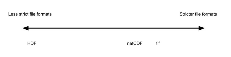
File Format Structure#
Concept No. 1: pros and cons of lenient file formats#
Pro |
Con |
|
|---|---|---|
Strict File Format |
easy to know what you’re going to get |
doesn’t handle all data types |
Not Strict File Format |
handles lots of data types |
what’s inside is unpredictable |
Concept No. 2: organizing variables by dimension#


Images from Fundamentals of NetCDF Storage by ESRI
When variables are defined in netCDF files they are also assigned dimensions. Dimensions tell us the axis over which our data varies. Common examples are latitute, longitude, or time. The values of the dimensions are given in special variables called coordinate variables. The coordinate variables and dimensions help us understand what the core data stored in each variable is describing. Attributes store metadata about our variables.
Concept No. 3: groups and datasets#
In the previous raster lessons we have been using data where the organization is a single dataset per file. HDF and netCDF are unique in that they allow multiple datasets to be in the same file. To keep organized, datasets are allowed to be stored together in groups. An analogy is to think of groups like folders in a folder structure and datasets as the individual files. Groups can have more groups inside of them.
HDF4#
Install#
In Anaconda Powershell:
conda install -c conda-forge -n lessons pyhdf
Documentation#
http://fhs.github.io/pyhdf/modules/SD.html (My opinion: pretty terrible docs)
Example dataset: CALIPSO#
CALIPSO Level 2: CAL_LID_L2_01kmCLay-Standard-V4-21.2020-07-01T07-32-43ZD.hdf
Opening the Dataset#
from pyhdf.SD import *
---------------------------------------------------------------------------
ModuleNotFoundError                       Traceback (most recent call last)
Cell In[1], line 1
----> 1 from pyhdf.SD import *

ModuleNotFoundError: No module named 'pyhdf'
filepath = './CAL_LID_L2_01kmCLay-Standard-V4-21.2020-07-01T07-32-43ZD.hdf'
# Opening the file
d = SD(filepath)
d
Exploring the dataset#
d.datasets()
Choose a key from the .datasets() dictionary and get the varaible info using .select()
d.select('Integrated_Attenuated_Backscatter_532')
Getting your data#
The data can be accessed using [:] and is output as a numpy array. Any of the methods we practiced with numpy arrays in lecture can be used on the dataset.
d.select('Integrated_Attenuated_Backscatter_532')[:]
backscatter = d.select('Integrated_Attenuated_Backscatter_532')[:]
type(backscatter)
backscatter.shape
backscatter.max()
Attributes#
Get metadata with the .attributes() method.
d.select('Integrated_Attenuated_Backscatter_532').attributes()
Masking a no data value#
While HDF5 data will automatically mask out nodata values, HDF4 datasets often don’t. To mask them yourself you can look up the fill value and apply it to the array.
import numpy.ma as ma
# Mask the array
masked_backscatter = ma.masked_where(backscatter == -9999, backscatter)
# Update the nodata value
ma.set_fill_value(backscatter, -9999)
masked_backscatter
HDF5#
Install#
In Anaconda Powershell:
conda install -c conda-forge -n lessons h5py
Documentation#
Example Dataset: ASTER Emissivity#
AG100.v003.83.-013.0001.h5
Attempting open with xarray#
# Returns empty
xr.open_dataset(filepath)
# Specify group.  If dataset is nested you can do /Emissivity/group2
xr.open_dataset(filepath, group='Emissivity')
# This also works for netCDF
<xarray.Dataset>
Dimensions:  (phony_dim_2: 5, phony_dim_3: 1000, phony_dim_4: 1000)
Dimensions without coordinates: phony_dim_2, phony_dim_3, phony_dim_4
Data variables:
    Mean     (phony_dim_2, phony_dim_3, phony_dim_4) int16 ...
SDev (phony_dim_2, phony_dim_3, phony_dim_4) int16 ...Opening a Dataset#
import h5py
filepath = './AG100.v003.83.-013.0001.h5'
f = h5py.File(filepath, 'r')
f
<HDF5 file "AG100.v003.83.-013.0001.h5" (mode r)>
Exploring Groups#
f.keys()
<KeysViewHDF5 ['ASTER GDEM', 'Emissivity', 'Geolocation', 'Land Water Map', 'NDVI', 'Observations', 'Temperature']>
f['Emissivity']
f['Emissivity'].keys()
f['Emissivity']['Mean']
You can check where you are in the file hierarchy with the .name method
f.name
f['Emissivity'].name
f['Emissivity']['Mean'].name
Getting your data#
The data inside the data group dictionaries are numpy arrays, so you can use any of the methods we learned about in other lectures with them.
mean_emissivity = f['Emissivity']['Mean'][:]
type(mean_emissivity)
mean_emissivity.shape
mean_emissivity.max()
from matplotlib import pyplot
pyplot.imshow(mean_emissivity[0])
Attributes#
Metadata in HDF files are called attributes and are accessed with .attrs
f['Emissivity']['Mean'].attrs.keys()
f['Emissivity']['Mean'].attrs['Description']
If there are no attributes for that group you will just get back an empty list
# No attributes on the Emissivity group
f['Emissivity'].attrs.keys()
# No attributes on the root group
f.attrs.keys()
netCDF#
Install#
In Anaconda Powershell:
conda install -c conda-forge -n lessons netcdf4
Documentation Link#
https://unidata.github.io/netcdf4-python/#creatingopeningclosing-a-netcdf-file
Example Dataset: MODIS Chlorophyll-a#
A2018006.L3m_DAY_CHL_chlor_a_4km.nc
Opening a Dataset - xarray#
notice comparing to panoply that “processing_control” is missing. Probs because its a group.
import xarray as xr
d_xr = xr.open_dataset(filepath)

d_xr
<xarray.Dataset>
Dimensions:  (lat: 4320, lon: 8640, rgb: 3, eightbitcolor: 256)
Coordinates:
  * lat      (lat) float32 89.98 89.94 89.9 89.85 ... -89.85 -89.9 -89.94 -89.98
  * lon      (lon) float32 -180.0 -179.9 -179.9 -179.9 ... 179.9 179.9 180.0
Dimensions without coordinates: rgb, eightbitcolor
Data variables:
    chlor_a  (lat, lon) float32 ...
    palette  (rgb, eightbitcolor) uint8 147 0 108 144 0 111 ... 105 0 0 0 0 0
Attributes: (12/64)
    product_name:                      A2018006.L3m_DAY_CHL_chlor_a_4km.nc
    instrument:                        MODIS
    title:                             MODISA Level-3 Standard Mapped Image
    project:                           Ocean Biology Processing Group (NASA/G...
    platform:                          Aqua
    temporal_range:                    day
    ...                                ...
    identifier_product_doi:            10.5067/AQUA/MODIS/L3M/CHL/2018
    keywords:                          Earth Science > Oceans > Ocean Chemist...
    keywords_vocabulary:               NASA Global Change Master Directory (G...
    data_bins:                         2440618
    data_minimum:                      0.0063775154
data_maximum: 98.49251xr.open_dataset(filepath, group='processing_control/input_parameters')
<xarray.Dataset>
Dimensions:  ()
Data variables:
    *empty*
Attributes: (12/29)
    par:               A2018006.L3m_DAY_CHL_chlor_a_4km.nc.param
    suite:             CHL
    ifile:             A2018006.L3b_DAY_CHL.nc
    ofile:             A2018006.L3m_DAY_CHL_chlor_a_4km.nc
    oformat:           2
    oformat2:          png
    ...                ...
    product_rgb:       rhos_645,rhos_555,rhos_469
    fudge:             1.0
    threshold:         0
    num_cache:         500
    mask_land:         no
land: $OCDATAROOT/common/landmask_GMT15ARC.ncOpening a Dataset - netCDF4#
from netCDF4 import Dataset
filepath = './A2018006.L3m_DAY_CHL_chlor_a_4km.nc'

d = Dataset(filepath, 'r')
Looking at the Dataset object gives us a decent overview of our dataset. We can see metadata applies to the whole dataset. At the very bottom the dimensions and varaiables are shown, as well as any additional groups.
d
<class 'netCDF4._netCDF4.Dataset'>
root group (NETCDF4 data model, file format HDF5):
    product_name: A2018006.L3m_DAY_CHL_chlor_a_4km.nc
    instrument: MODIS
    title: MODISA Level-3 Standard Mapped Image
    project: Ocean Biology Processing Group (NASA/GSFC/OBPG)
    platform: Aqua
    temporal_range: day
    processing_version: 2018.0
    date_created: 2018-03-19T18:42:34.000Z
    history: l3mapgen par=A2018006.L3m_DAY_CHL_chlor_a_4km.nc.param
    l2_flag_names: ATMFAIL,LAND,HILT,HISATZEN,STRAYLIGHT,CLDICE,COCCOLITH,LOWLW,CHLWARN,CHLFAIL,NAVWARN,MAXAERITER,ATMWARN,HISOLZEN,NAVFAIL,FILTER,HIGLINT
    time_coverage_start: 2018-01-06T00:15:01.000Z
    time_coverage_end: 2018-01-07T02:30:00.000Z
    start_orbit_number: 83382
    end_orbit_number: 83397
    map_projection: Equidistant Cylindrical
    latitude_units: degrees_north
    longitude_units: degrees_east
    northernmost_latitude: 90.0
    southernmost_latitude: -90.0
    westernmost_longitude: -180.0
    easternmost_longitude: 180.0
    geospatial_lat_max: 90.0
    geospatial_lat_min: -90.0
    geospatial_lon_max: 180.0
    geospatial_lon_min: -180.0
    grid_mapping_name: latitude_longitude
    latitude_step: 0.041666668
    longitude_step: 0.041666668
    sw_point_latitude: -89.979164
    sw_point_longitude: -179.97917
    geospatial_lon_resolution: 4.6383123
    geospatial_lat_resolution: 4.6383123
    geospatial_lat_units: degrees_north
    geospatial_lon_units: degrees_east
    spatialResolution: 4.64 km
    number_of_lines: 4320
    number_of_columns: 8640
    measure: Mean
    suggested_image_scaling_minimum: 0.01
    suggested_image_scaling_maximum: 20.0
    suggested_image_scaling_type: LOG
    suggested_image_scaling_applied: No
    _lastModified: 2018-03-19T18:42:34.000Z
    Conventions: CF-1.6 ACDD-1.3
    institution: NASA Goddard Space Flight Center, Ocean Ecology Laboratory, Ocean Biology Processing Group
    standard_name_vocabulary: CF Standard Name Table v36
    naming_authority: gov.nasa.gsfc.sci.oceandata
    id: A2018006.L3b_DAY_CHL.nc/L3/A2018006.L3b_DAY_CHL.nc
    license: http://science.nasa.gov/earth-science/earth-science-data/data-information-policy/
    creator_name: NASA/GSFC/OBPG
    publisher_name: NASA/GSFC/OBPG
    creator_email: data@oceancolor.gsfc.nasa.gov
    publisher_email: data@oceancolor.gsfc.nasa.gov
    creator_url: http://oceandata.sci.gsfc.nasa.gov
    publisher_url: http://oceandata.sci.gsfc.nasa.gov
    processing_level: L3 Mapped
    cdm_data_type: grid
    identifier_product_doi_authority: http://dx.doi.org
    identifier_product_doi: 10.5067/AQUA/MODIS/L3M/CHL/2018
    keywords: Earth Science > Oceans > Ocean Chemistry > Pigments > Chlorophyll; Earth Science > Oceans > Ocean Chemistry > Chlorophyllr
    keywords_vocabulary: NASA Global Change Master Directory (GCMD) Science Keywords
    data_bins: 2440618
    data_minimum: 0.0063775154
    data_maximum: 98.49251
    dimensions(sizes): lat(4320), lon(8640), rgb(3), eightbitcolor(256)
    variables(dimensions): float32 chlor_a(lat, lon), float32 lat(lat), float32 lon(lon), uint8 palette(rgb, eightbitcolor)
    groups: processing_control
You can also directly access dimensions or varaiables. The outputs act like dictionaries, so you can use .keys() or [KEY] syntax to access elements
d.dimensions
d.variables
{'chlor_a': <class 'netCDF4._netCDF4.Variable'>
 float32 chlor_a(lat, lon)
     long_name: Chlorophyll Concentration, OCI Algorithm
     units: mg m^-3
     standard_name: mass_concentration_chlorophyll_concentration_in_sea_water
     _FillValue: -32767.0
     valid_min: 0.001
     valid_max: 100.0
     reference: Hu, C., Lee Z., and Franz, B.A. (2012). Chlorophyll-a algorithms for oligotrophic oceans: A novel approach based on three-band reflectance difference, J. Geophys. Res., 117, C01011, doi:10.1029/2011JC007395.
     display_scale: log
     display_min: 0.01
     display_max: 20.0
 unlimited dimensions:
 current shape = (4320, 8640)
 filling on,
 'lat': <class 'netCDF4._netCDF4.Variable'>
 float32 lat(lat)
     long_name: Latitude
     units: degrees_north
     standard_name: latitude
     _FillValue: -999.0
     valid_min: -90.0
     valid_max: 90.0
 unlimited dimensions:
 current shape = (4320,)
 filling on,
 'lon': <class 'netCDF4._netCDF4.Variable'>
 float32 lon(lon)
     long_name: Longitude
     units: degrees_east
     standard_name: longitude
     _FillValue: -999.0
     valid_min: -180.0
     valid_max: 180.0
 unlimited dimensions:
 current shape = (8640,)
 filling on,
 'palette': <class 'netCDF4._netCDF4.Variable'>
 uint8 palette(rgb, eightbitcolor)
 unlimited dimensions:
 current shape = (3, 256)
 filling on, default _FillValue of 255 ignored}
# Treating a variable like a dictionary
print(d.variables.keys())
d.variables['chlor_a']
dict_keys(['chlor_a', 'lat', 'lon', 'palette'])
<class 'netCDF4._netCDF4.Variable'>
float32 chlor_a(lat, lon)
    long_name: Chlorophyll Concentration, OCI Algorithm
    units: mg m^-3
    standard_name: mass_concentration_chlorophyll_concentration_in_sea_water
    _FillValue: -32767.0
    valid_min: 0.001
    valid_max: 100.0
    reference: Hu, C., Lee Z., and Franz, B.A. (2012). Chlorophyll-a algorithms for oligotrophic oceans: A novel approach based on three-band reflectance difference, J. Geophys. Res., 117, C01011, doi:10.1029/2011JC007395.
    display_scale: log
    display_min: 0.01
    display_max: 20.0
unlimited dimensions:
current shape = (4320, 8640)
filling on
# Access metadata with using a period .
d.variables['chlor_a'].long_name
If the data you need is in a group, it can be accessed with .groups
d.groups['processing_control']
<class 'netCDF4._netCDF4.Group'>
group /processing_control:
    software_name: l3mapgen
    software_version: 2.0.0-V2018.0.6
    source: A2018006.L3b_DAY_CHL.nc
    l2_flag_names: ATMFAIL,LAND,HILT,HISATZEN,STRAYLIGHT,CLDICE,COCCOLITH,LOWLW,CHLWARN,CHLFAIL,NAVWARN,MAXAERITER,ATMWARN,HISOLZEN,NAVFAIL,FILTER,HIGLINT
    dimensions(sizes):
    variables(dimensions):
    groups: input_parameters
Getting your data#
Once you traverse the file structure with the right keys and find a netCDF4._netCDF4.Variable object you can accesss pull out the numpy array and work with it.
chlor_a = d.variables['chlor_a'][:]
type(chlor_a)
chlor_a.shape
chlor_a.max()
from matplotlib import pyplot
pyplot.imshow(chlor_a)