Working with rasters#
Lesson Content
🧠Anatomy of a raster
📖Opening a file
🔍Inspecting the metadata
🚜Working with the data
💾Saving a file
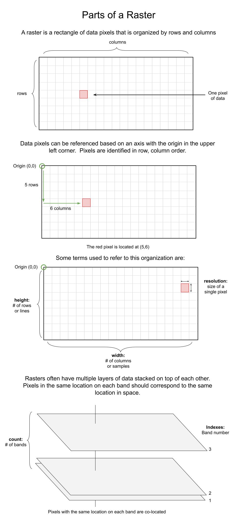
🧠 The Anatomy of a raster#
Working with raster data involves understanding how rasters are organized.
📝 Check your understanding
You open a raster file and see that the count is 224. What have you just learned about the raster?
📖 Opening a file#
When you open data files in Python you usually need to use a library. When dealing with raster data there are several common libraries, most of which cater to a specific data type:
File Format |
File Extension |
Python Library |
|---|---|---|
netCDF |
|
netCDF4 |
HDF5 |
|
h5py |
HDF4 |
|
pyhdf |
geoTIFF |
|
rasterio |
zarr |
|
zarr |
While each of these libraries works best with their associated file type, I really like to use rasterio because it does a particularly good job of accomodating many data types. I usually start with rasterio and switch to the a different file-specific library only if I need something extra rasterio doesn’t already provide.
Opening a file with rasterio#
We open our rasters with the rasterio.open() method. The general syntax is
with rasterio.open(FILEPATH_TO_RASTER, DATAMODE) as src:
   print(src)
where FILEPATH_TO_RASTER is the place on your computer where the data is stored and DATAMODE is usually either ‘r’ for read (opening existing data) or ‘w’ for write (creating new data). There are other data modes but these are two very common ones.
An example of opening a file using test AVIRIS data:
# Define the filepath to our raster
filepath_rad = './data/subset_f180628t01p00r02_corr_v1k1_img'
Filepaths#
Ahe filepath and is a string that describes the location of the data that you want to open. A few pieces of the anatomy of a filepath to notice:
/- forward slashes signal that you have entered a new folder..- the period at the beginning tells the computer to start looking for data in the same place tht the code is being run in.
Choosing to start your filepath with a . is called specificying a relative filepath, because you are telling the computer to start looking for the file relative to where the file is being run. If you move this file to another place on your computer and don’t move the data with it the import statment won’t work anymore. The alternative to a relative filepath is an aboslute filepath, in which case you start your file path at the very tippy top of your computer’s organizational structure (the root directory).
Other vocab notes:
directory is the same thing as a folder.
To loop back to our example, we put together our filepath by defining the following directions for our computer:
start by specifing the current directory as the starting point:
.go into the data folder:
./datachoose the file named “subset_f180628t01p00r02_corr_v1k1_img”:
'./data/subset_f180628t01p00r02_corr_v1k1_img'
🎉 And there we have our file
import rasterio
# Open the file
with rasterio.open(filepath_rad, 'r') as src:
    print(src)
<open DatasetReader name='./data/subset_f180628t01p00r02_corr_v1k1_img' mode='r'>
The object that gets returned here <open DatasetReader name='./data/subset_f180628t01p00r02_corr_v1k1_img' mode='r'> is the “Dataset Reader” object. This object connects you to the file in Python, but it isn’t actually the data. To get to the data you need to use src.read().
Reading a raster band with rasterio#
General syntax:
with rasterio.open(FILEPATH_TO_RASTER, DATAMODE) as src:
   print(src.read(BAND_INDEX))
where FILEPATH_TO_RASTER is the place on your computer where the data is DATAMODE is usually either ‘r’ for read (opening existing data) or ‘w’ for write (creating new data). BAND_INDEX indicates which band you want to read. Leaving BAND_INDEX blank reads the entire raster (all bands).
An example:
# Reading the first band from our file
with rasterio.open(filepath_rad, 'r') as src:
    print(src.read(5))
[[-8.8028395e-01 -8.8028395e-01 -8.8028395e-01 ...  7.7182706e-04
   1.8142069e-02  2.4249963e-02]
 [-8.8028395e-01 -8.8028395e-01 -8.8028395e-01 ...  1.2664238e-02
   1.7274955e-02  2.1294061e-02]
 [-8.8028395e-01 -8.8028395e-01 -8.8028395e-01 ...  1.6278537e-02
   1.4166061e-02  1.2966915e-02]
 ...
 [-8.8028395e-01 -8.8028395e-01 -8.8028395e-01 ...  3.9758585e-02
   3.6750916e-02  4.9293626e-02]
 [-8.8028395e-01 -8.8028395e-01 -8.8028395e-01 ...  4.6895660e-02
   5.5631310e-02  4.7900975e-02]
 [-8.8028395e-01 -8.8028395e-01 -8.8028395e-01 ...  5.4747202e-02
   5.0485637e-02  5.1755313e-02]]
What gets printed here are our actual data values! 🎉
Getting a quick visual of the data#
Another way to quickly get eyes on our data is to use the show command.
from matplotlib import pyplot
with rasterio.open(filepath_rad, 'r') as src:
    pyplot.imshow(src.read(5))
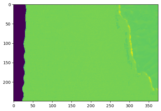
The plot and the array might not be very useful right now, but at least we have validated that we can open our raster and that it contains data.
If you like viewing quick plots as a way of interacting with your data you can read more about it in the rasterio docs.
🌀 More Info: Context managers
It might be new to you that I used the syntax:
with ... as src:
    src.read()
This syntax is called the Context manager. When we read files we are opening them up, like a book, and they stay open until we tell the program to close them. The benefit of the context manager is that it opens up a file when you use the with statement, runs all your lines of indented code, and the closes the file after. This is important if you are opening up large files. Your computer only has so much memory, so if you try to open too many 8GB files at once without closing them you can crash your program.
If you don’t want to use the contect manager another way to this same task is to run:
src = rasterio.open(filepath_rad, 'r')
src.read(1)
print(src)
src.close()
If you do this, though, make sure to only be working with a few files at a time or to close your files.
📝 Check your understanding
What is happening in the following piece of code? How many bands will be affected?
with rasterio.open('./data/f180628t01p00r02_corr_v1k1_img', 'r') as src:
    src.read()
🔍 Inspecting the Metadata#
When you first open a dataset it is often helpful to get your bearings by inspecting the metadata. In rasterio we do this by inspecting the DatasetReader object (src) that was returned when you opened the object.
There are lots of attributes that you check a dataset reader for. If you want to get an general overview I like to use src.meta. To extract specific values here are some more attributes that I find useful:
src.bounds- Returns the lower left and upper right bounds of the dataset in the units of its coordinate reference system. (lower left x, lower left y, upper right x, upper right y)src.count- The number of raster bands in the datasetsrc.crs- The dataset’s coordinate reference systemsrc.descriptions- Descriptions for each dataset bandsrc.dtypes- The data types of each band in index ordersrc.height- The number of pixels in each columnsrc.indexes- The 1-based indexes of each band in the datasetsrc.meta- The basic metadata of this dataset.src.name- Relative filepath of the datasetsrc.nodata- The dataset’s single nodata valuesrc.res- Returns the (width, height) of pixels in the units of its coordinate reference system.src.transform- The dataset’s georeferencing transformation matrixsrc.units- one units string for each dataset bandsrc.width- the number of pixels in each row
All of the parts of the raster that were addressed in the first section of this notebook Anatomy of a raster are accessible using these attributes.
Example#
# Try substituting any of the above attributes in for this dataset
with rasterio.open(filepath_rad, 'r') as src:
    print(src.meta)
{'driver': 'ENVI', 'dtype': 'float32', 'nodata': None, 'width': 375, 'height': 250, 'count': 224, 'crs': CRS.from_epsg(32610), 'transform': Affine(1.02258007728804e-15, 16.7, 769855.79,
       16.7, -1.02258007728804e-15, 3751257.6)}
with rasterio.open(filepath_rad, 'r') as src:
    print(src.read().shape)
(224, 250, 375)
With the above print statement we learned from the src.meta information that the raster has 224 bands (count) it has the coordinate reference system EPSG code 32610 (crs), it is an ENVI filetype (driver), the datatype is float32 (dtype), it has 250 rows or is 250 pixels tall (height), there isn’t a nodata value set (nodata), the affine tranform is (1.02258007728804e-15, 16.7, 769855.79, 16.7, -1.02258007728804e-15, 3751257.6) (tranform), and that the raster has 375 columns or is 375 pixels wide. We also see the relative filepath of the raster from the src.name attribute.
📝 Check your understanding
Which of the following are metadata in an AVIRIS reflectance dataset?
A) Number of bands
B) Coordinate information
C) Reflectance values
D) Height/Lines and Width/Samples
Answer with all of the letters that are metadata.
🚜 Working with the Data#
While the raster file is is accessed through a unique filetype-specific library, the actual data is almost always just a common matrix datatype. Numpy is the most common library used, but xarray is also used by some data libraries.
This means that everything we working on last week for matricies applies to the data inside the raster file.
with rasterio.open(filepath_rad, 'r') as src:
    red_band = src.read(50)
    blue_band = src.read(10)
    green_band = src.read(20)
Indexing#
A reminder about matrix indexing:
2D matrices use row, column order
3D matrices use height, row, column order
red_band[249, 374]
0.005221703
red_band[144, 100]
0.0062336302
# One long row of data
red_band[4]
array([-9.89863992e-01, -9.89863992e-01, -9.89863992e-01, -9.89863992e-01,
       -9.89863992e-01, -9.89863992e-01, -9.89863992e-01, -9.89863992e-01,
       -9.89863992e-01, -9.89863992e-01, -9.89863992e-01, -9.89863992e-01,
       -9.89863992e-01, -9.89863992e-01, -9.89863992e-01, -9.89863992e-01,
       -9.89863992e-01, -9.89863992e-01, -9.89863992e-01, -9.89863992e-01,
       -9.89863992e-01, -9.89863992e-01, -9.89863992e-01, -9.89863992e-01,
       -9.89863992e-01, -9.89863992e-01, -9.89863992e-01, -9.89863992e-01,
       -9.89863992e-01, -9.89863992e-01, -9.89863992e-01, -9.89863992e-01,
        9.60341003e-03,  8.56745243e-03,  9.77658853e-03,  1.21959150e-02,
        1.21608926e-02,  1.01511301e-02,  1.22256568e-02,  1.22256568e-02,
        9.97462496e-03,  1.32317590e-02,  9.90260020e-03,  7.78485741e-03,
        1.16055440e-02,  1.03626624e-02,  1.03626624e-02,  8.48274026e-03,
        1.07032945e-02,  1.05163530e-02,  5.99020347e-03,  9.29890200e-03,
        1.20315310e-02,  8.23581219e-03,  8.52218829e-03,  8.52218829e-03,
        9.99249145e-03,  1.08621847e-02,  1.27621852e-02,  9.74960625e-03,
        9.93011892e-03,  1.10991010e-02,  9.72998329e-03,  9.72998329e-03,
        1.37429517e-02,  1.07355947e-02,  1.04636298e-02,  1.22513892e-02,
        1.17190378e-02,  9.16020479e-03,  1.16725871e-02,  1.16725871e-02,
        9.93436389e-03,  9.92709771e-03,  7.87495449e-03,  9.22061317e-03,
        1.08120767e-02,  1.17061716e-02,  7.62484455e-03,  7.62484455e-03,
        1.27769317e-02,  1.16161704e-02,  1.13528278e-02,  9.19037219e-03,
        1.14430059e-02,  1.06365317e-02,  7.00194389e-03,  9.92375892e-03,
        1.04948664e-02,  1.04948664e-02,  9.83347651e-03,  4.01473558e-03,
        1.02585070e-02,  6.51265541e-03,  3.85753764e-03,  1.37749342e-02,
        1.18129533e-02,  1.18129533e-02,  1.16536515e-02,  8.72882642e-03,
        1.08521413e-02,  1.13936057e-02,  1.24934735e-02,  1.01565169e-02,
        7.94219784e-03,  1.11402711e-02,  1.11402711e-02,  1.07124457e-02,
        9.70683526e-03,  9.39665642e-03,  1.11531522e-02,  1.22633809e-02,
        1.00097349e-02,  1.03047434e-02,  1.22710364e-02,  7.45117245e-03,
        8.91800411e-03,  8.91800411e-03,  1.00032743e-02,  1.03893792e-02,
        1.14607411e-02,  1.13273570e-02,  9.52258985e-03,  1.04254112e-02,
        9.68714152e-03,  7.56124547e-03,  7.56124547e-03,  9.12059192e-03,
        1.15978923e-02,  8.94551259e-03,  9.03818756e-03,  1.14348466e-02,
        1.12770488e-02,  1.01099340e-02,  1.09425560e-02,  1.27936015e-02,
        1.03212325e-02,  1.20040122e-02,  1.15839001e-02,  1.09657971e-02,
        1.08133005e-02,  1.14410305e-02,  1.02785453e-02,  1.22435279e-02,
        1.13794953e-02,  1.03773763e-02,  1.46823423e-02,  1.31757027e-02,
        1.31757027e-02,  1.34336296e-02,  1.34091042e-02,  1.01813180e-02,
        7.18480861e-03,  1.32976491e-02,  9.29967128e-03,  9.34869051e-03,
        8.52198992e-03,  8.50201119e-03,  8.50201119e-03,  1.13882786e-02,
        8.57987348e-03,  8.28727987e-03,  1.09522119e-02,  8.20450671e-03,
        1.02974121e-02,  9.24416911e-03,  1.05280252e-02,  9.57950391e-03,
        9.75759793e-03,  9.37086716e-03,  9.37086716e-03,  8.56183190e-03,
        9.64759290e-03,  1.14238849e-02,  7.76233617e-03,  7.44129391e-03,
        5.89989871e-03,  6.99818227e-03,  8.07397719e-03,  7.37830950e-03,
        5.37360925e-03,  7.98865873e-03,  7.98865873e-03,  5.78207243e-03,
        3.37526924e-03,  1.02493092e-02,  8.17018934e-03,  5.70513587e-03,
        9.31401737e-03,  5.99309057e-03,  1.04032306e-03,  2.40463717e-03,
        7.23264366e-03,  6.07277872e-03,  7.87939131e-03,  7.87939131e-03,
        5.02707716e-03,  1.04341060e-02,  6.54117577e-03,  6.40173163e-03,
        8.48427694e-03,  9.44371521e-03,  1.09653706e-02,  8.80982541e-03,
        8.23528913e-04,  5.77815436e-03,  1.14251103e-03,  1.14251103e-03,
        5.72341774e-03,  7.61449104e-03,  5.68367587e-03,  1.26515748e-02,
        5.33479173e-03,  6.80172350e-03,  8.36720411e-03,  7.88195804e-03,
        1.25120173e-03,  1.03334403e-02,  9.92541667e-03,  1.33938612e-02,
        1.33938612e-02,  7.69980485e-03,  9.40576103e-03,  5.77459997e-03,
        6.79657003e-03,  1.15214370e-03,  4.47639171e-03,  1.15755051e-02,
        8.78010783e-03,  8.72862712e-03,  9.10193846e-03,  5.86174522e-03,
        6.20170590e-03,  5.15950611e-03,  4.94923256e-03,  4.94923256e-03,
        7.73387915e-03,  6.25468977e-03,  7.82719348e-03,  6.18605362e-03,
        5.79997199e-03,  8.95670056e-03,  8.15831777e-03,  1.17874248e-02,
        5.76946558e-03,  7.13090133e-03,  4.88395710e-03,  2.29153968e-03,
        7.00125797e-03,  5.55184297e-03,  5.44924103e-03,  5.44924103e-03,
        5.80242230e-03,  8.49946123e-03,  7.27876043e-03,  9.87273734e-03,
        6.17004791e-03,  4.39421041e-03,  3.98266455e-03,  6.80908607e-03,
        8.64381902e-03,  7.45708495e-03,  5.65337949e-03,  7.08853174e-03,
        9.51331947e-03,  9.51331947e-03,  1.79716554e-02,  6.48755431e-02,
        1.11067332e-01,  3.25312838e-02,  1.32159684e-02,  1.57204792e-02,
        1.82487592e-02,  2.96701975e-02,  9.13888589e-02,  1.68310538e-01,
        2.26290867e-01,  1.68618903e-01,  1.52089566e-01,  1.53015971e-01,
        1.71361595e-01,  1.71361595e-01,  1.78749010e-01,  1.68540463e-01,
        1.47794291e-01,  1.26275867e-01,  1.13734059e-01,  1.01421140e-01,
        8.83982405e-02,  9.72591266e-02,  1.32041112e-01,  1.59027189e-01,
        1.94381401e-01,  2.22682908e-01,  2.15925947e-01,  2.15925947e-01,
        2.29753554e-01,  2.33850136e-01,  2.35325441e-01,  2.55388141e-01,
        2.82413244e-01,  3.10377479e-01,  3.28700691e-01,  2.59206623e-01,
        2.51021773e-01,  2.54293412e-01,  2.89322555e-01,  3.31567198e-01,
        3.36291105e-01,  3.10564101e-01,  3.10564101e-01,  2.74938077e-01,
        2.63735503e-01,  2.59882569e-01,  2.79308110e-01,  2.56433010e-01,
        2.47580290e-01,  2.55837888e-01,  2.67711788e-01,  2.15465501e-01,
        1.56197593e-01,  1.37191728e-01,  1.23051502e-01,  1.19016066e-01,
        1.14996009e-01,  1.30868509e-01,  1.41310662e-01,  1.41310662e-01,
        1.36986896e-01,  1.45302624e-01,  1.62975192e-01,  1.80153936e-01,
        2.03104600e-01,  1.95680529e-01,  2.11470127e-01,  2.07485899e-01,
        1.85355276e-01,  1.83796972e-01,  1.77590415e-01,  1.59322709e-01,
        1.48297369e-01,  1.56327918e-01,  1.51601136e-01,  1.51601136e-01,
        1.54474974e-01,  1.83645815e-01,  2.62981385e-01,  2.58784413e-01,
        1.68838456e-01,  1.10366546e-01,  9.83937159e-02,  8.98709968e-02,
        7.62339979e-02,  1.12549394e-01,  1.21540807e-01,  1.02702200e-01,
        1.04190111e-01,  1.32186681e-01,  1.56810403e-01,  1.60454646e-01,
        1.45415485e-01,  1.29735738e-01,  1.34829611e-01,  1.46270335e-01,
        1.47036850e-01,  1.60749197e-01,  1.60749197e-01,  1.77667767e-01,
        1.45186886e-01,  1.20232992e-01,  1.24302126e-01,  1.59918860e-01,
        1.74745366e-01,  1.62464723e-01,  9.29672793e-02], dtype=float32)
Exploratory statistics#
When I open a dataset I often like to get a sense of it by just looking at looking at statistics for one of the bands. We can use the aggregation functions from last week for this.
print('max value: ', green_band.max())
print('mean value: ', green_band.mean())
print('min value: ', green_band.min())
max value:  0.4638913
mean value:  -0.037566137
min value:  -0.9919098
Matrix Operations#
Adding and subtracting two matrices
red_band + green_band
array([[-1.9817739 , -1.9817739 , -1.9817739 , ...,  0.13850516,
         0.20546283,  0.33700895],
       [-1.9817739 , -1.9817739 , -1.9817739 , ...,  0.18310083,
         0.27180833,  0.28681755],
       [-1.9817739 , -1.9817739 , -1.9817739 , ...,  0.28129148,
         0.29883683,  0.23306896],
       ...,
       [-1.9817739 , -1.9817739 , -1.9817739 , ...,  0.04379314,
         0.04434666,  0.04983609],
       [-1.9817739 , -1.9817739 , -1.9817739 , ...,  0.04094062,
         0.05011846,  0.04768296],
       [-1.9817739 , -1.9817739 , -1.9817739 , ...,  0.05058881,
         0.04569351,  0.04583649]], dtype=float32)
blue_band - red_band
array([[ 0.03121787,  0.03121787,  0.03121787, ..., -0.06602393,
        -0.11272857, -0.20093265],
       [ 0.03121787,  0.03121787,  0.03121787, ..., -0.0920296 ,
        -0.15151955, -0.14239667],
       [ 0.03121787,  0.03121787,  0.03121787, ..., -0.15002072,
        -0.17034033, -0.11561722],
       ...,
       [ 0.03121787,  0.03121787,  0.03121787, ...,  0.04716351,
         0.04572179,  0.05058041],
       [ 0.03121787,  0.03121787,  0.03121787, ...,  0.05341611,
         0.05365299,  0.05151878],
       [ 0.03121787,  0.03121787,  0.03121787, ...,  0.05188685,
         0.05395792,  0.0552441 ]], dtype=float32)
Multiplying or dividing a matrix by a constant
red_band*5
array([[-4.94932   , -4.94932   , -4.94932   , ...,  0.4822076 ,
         0.768427  ,  1.2765377 ],
       [-4.94932   , -4.94932   , -4.94932   , ...,  0.6515627 ,
         1.0018888 ,  1.0037379 ],
       [-4.94932   , -4.94932   , -4.94932   , ...,  1.0025584 ,
         1.0973514 ,  0.81842124],
       ...,
       [-4.94932   , -4.94932   , -4.94932   , ...,  0.02871939,
         0.03346157,  0.04347686],
       [-4.94932   , -4.94932   , -4.94932   , ...,  0.01182676,
         0.04153725,  0.03549127],
       [-4.94932   , -4.94932   , -4.94932   , ...,  0.05110819,
         0.02780656,  0.02610851]], dtype=float32)
green_band/7
array([[-0.1417014 , -0.1417014 , -0.1417014 , ...,  0.00600909,
         0.00739677,  0.01167163],
       [-0.1417014 , -0.1417014 , -0.1417014 , ...,  0.00754119,
         0.01020437,  0.01229571],
       [-0.1417014 , -0.1417014 , -0.1417014 , ...,  0.01153998,
         0.01133808,  0.0099121 ],
       ...,
       [-0.1417014 , -0.1417014 , -0.1417014 , ...,  0.00543561,
         0.00537919,  0.00587725],
       [-0.1417014 , -0.1417014 , -0.1417014 , ...,  0.00551075,
         0.005973  ,  0.00579782],
       [-0.1417014 , -0.1417014 , -0.1417014 , ...,  0.00576674,
         0.00573317,  0.00580211]], dtype=float32)
Some other built in operations
import numpy as np
# We have to take the absolute value of red because the nodata values are negative
# and that throws an error
np.sqrt(abs(red_band))
array([[0.99491906, 0.99491906, 0.99491906, ..., 0.31055036, 0.3920273 ,
        0.50527966],
       [0.99491906, 0.99491906, 0.99491906, ..., 0.36098826, 0.44763574,
        0.44804865],
       [0.99491906, 0.99491906, 0.99491906, ..., 0.4477853 , 0.46847656,
        0.4045791 ],
       ...,
       [0.99491906, 0.99491906, 0.99491906, ..., 0.07578838, 0.08180656,
        0.09324898],
       [0.99491906, 0.99491906, 0.99491906, ..., 0.04863489, 0.09114521,
        0.08425114],
       [0.99491906, 0.99491906, 0.99491906, ..., 0.10110211, 0.07457421,
        0.07226136]], dtype=float32)
np.power(red_band, 5)
array([[-9.50336993e-01, -9.50336993e-01, -9.50336993e-01, ...,
         8.34296225e-06,  8.57359846e-05,  1.08472107e-03],
       [-9.50336993e-01, -9.50336993e-01, -9.50336993e-01, ...,
         3.75777636e-05,  3.23033426e-04,  3.26025620e-04],
       [-9.50336993e-01, -9.50336993e-01, -9.50336993e-01, ...,
         3.24114313e-04,  5.09188452e-04,  1.17499076e-04],
       ...,
       [-9.50336993e-01, -9.50336993e-01, -9.50336993e-01, ...,
         6.25210387e-12,  1.34239833e-11,  4.97096496e-11],
       [-9.50336993e-01, -9.50336993e-01, -9.50336993e-01, ...,
         7.40421450e-14,  3.95674951e-11,  1.80201236e-11],
       [-9.50336993e-01, -9.50336993e-01, -9.50336993e-01, ...,
         1.11584131e-10,  5.31969304e-12,  3.88204789e-12]], dtype=float32)
There are lots more built in functions. This table has a nice list.
Plotting#
Also notice that plotting works for a single band
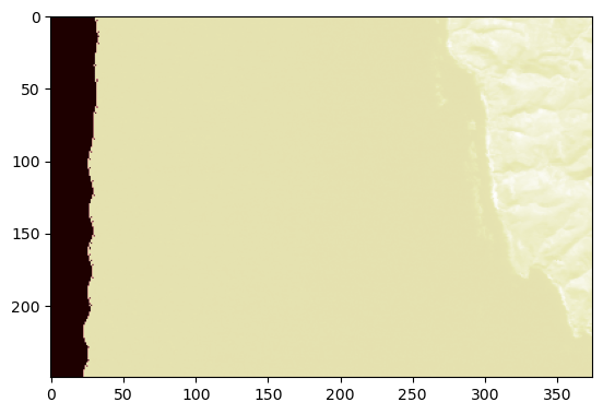
pyplot.imshow(red_band, cmap='pink')
<matplotlib.image.AxesImage at 0x10877d4e0>
📝 Check your understanding
Say that the variable reflectance hold all of the data for an AVIRIS raster – count 224 with 1000 rows and 350 columns.
What is the index you need to use to get the all the data for band 100?
💾 Saving a file#
At a certain point you may want to do it. Let’s start by getting some data to save
# Get our data setup
with rasterio.open(filepath_rad, 'r') as src:
    red_src = src.read(50)
    blue_src = src.read(20)
    green_src = src.read(10)
    meta = src.meta.copy()
It is best practice to persist or update as much of the metadata from your old raster as you can. As you may have experienced working with data, complete and accurate metadata can make someone else’s life (and maybe even your own) much easier down the road. Make sure you look at it, though, to make sure all the information still applies to your new raster.
Count has changed, since we are only saving 3 of the 224 total bands, so we need to upadate the count value. I am also going to set -50 as the nodata value.
meta['count'] = 3
Another thing you could do is add tags to your bands so that you remember what band number you used. You do this when you write out the data.
# Make the output directory if it does not exist yet
import os
if not os.path.exists('../output_data'):
    os.makedirs('../output_data')
with rasterio.open(
    '../output_data/rgb',
    'w',
    **meta
) as dst:
    # Write data matrices
    dst.write(red_src, 1)
    dst.write(green_src, 2)
    dst.write(blue_src, 3)
    # Add band tags
    dst.update_tags(1, src_band=50)
    dst.update_tags(2, src_band=10)
    dst.update_tags(3, src_band=20)
If we want to confirm that our dataset saved properly we can open it back up and look at what we saved.
with rasterio.open('../output_data/rgb', 'r') as src:
    red_dst = src.read(1)
    green_dst = src.read(2)
    blue_dst = src.read(3)
print('Source stats: ')
print('red: ', red_src.mean(), red_src.max())
print('green: ', green_src.mean(), green_src.max())
print('blue: ', blue_src.mean(), blue_src.max())
print('Destination stats: ')
print('red: ', red_dst.mean(), red_dst.max())
print('green: ', green_dst.mean(), green_dst.max())
print('blue: ', blue_dst.mean(), blue_dst.max())
Source stats:
red:  -0.043670043 0.40461412
green:  -0.022554584 0.41501164
blue:  -0.037566137 0.4638913
Destination stats:
red:  -0.043670043 0.40461412
green:  -0.022554584 0.41501164
blue:  -0.037566137 0.4638913
Our values line up! And the new values came from the raster we made ourselves. 😄