The pandas Library

Lesson Content

• 🗃️ Libraries

• 🐼 pandas Data structures

• 🔍 Accessing values in DataFrames

• 💧 Filepaths & Opening files with USGS stream gauge data

• 👨‍👦‍👦 Some Aggregations

Context

Today we are building up our arsenal of data structures with a really exciting one - the pandas Dataframe. This is a data structure that models tabular data, or data with labelled rows and columns. Learning this data structure will allow us to start manipulating large datasets of that format, and do things that we couldn’t otherwise do in a program like excel.

Today we will focus on opening and inspecting data, using USGS stream gauge data as an applied example.

🗃️ Libraries

Today we are going to dig into our first library in Python! A library is a like an “extras” package for a programming language (think Settlers of Catan expansion pack). It is a set of commands that doesn’t automatically come activated when you use Python, but that you can still use if you just tell Python that you plan to do so. You let python know you are going to use a library with an import statment. After you do that the additional commands become availble.

# Attempting to use the `math` library before importing
math.factorial(3)

---------------------------------------------------------------------------
NameError                                 Traceback (most recent call last)
Cell In[1], line 2
      1 # Attempting to use the `math` library before importing
----> 2 math.factorial(3)

NameError: name 'math' is not defined

# Importing a Python library
import math

# Attempt #2 to use the `math` libray, after importing
math.factorial(3)

6

Once we have imported the library we can use the new commands that the library contains. The math library was just an example and it isn’t the focus of this lesson, but if you want you can see a list of math commands here.

🌀 More Info: Standard vs. Non-standard Libraries

One large chunk of libraries are together referred to as the Python Standard Library. These libraries are not a part of the “core” language (everything we can do without import statments) but have still been offically accepted into the Python distribution package and are maintained in the same way as the rest of the core language. You can read more here.

There are also libraries which aren’t a part of this designation, and are still widely used and developed, but they are simply not included when you hit the “Download Python” button. Non-standard libraries are maintained by groups of developers outside of the Python Software Foundation and anyone can make one. That includes you!

🐼 Tabular Data and pandas

Tabular data is the type of data that you would see in an excel sheet. Data is organized into rows (horizontal) and columns (vertical). It is also common for tabular data to have an index which uniquely lables the rows. A really common type of tabular data is a CSV file.

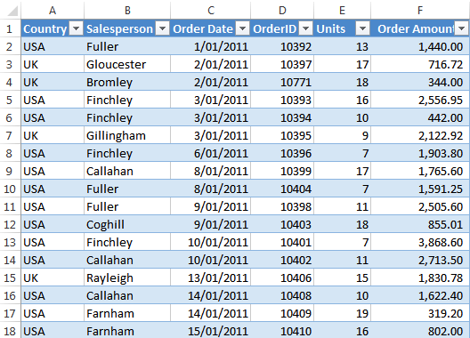
Where are the rows, columns, and indexes in this excel sheet?

pandas library 🐼

pandas is a very common library that is used for working with tabular data. It is cannonically imported like this:

# Import the libary.  You only have to do this once per file.
import pandas as pd

# This line shortens the output. It will be explained more later in the notebook.
pd.set_option('display.max_rows', 10)
pd.set_option('display.max_columns', 6)

pandas Data structures

There are two primary pandas data structures:

1. pd.Series

2. pd.DataFrame

The primary structure of these two is a DataFrame and a Series is a simpler version of a DataFrame. Knowing that both exist, however, can be helpful when debugging.

pd.DataFrame

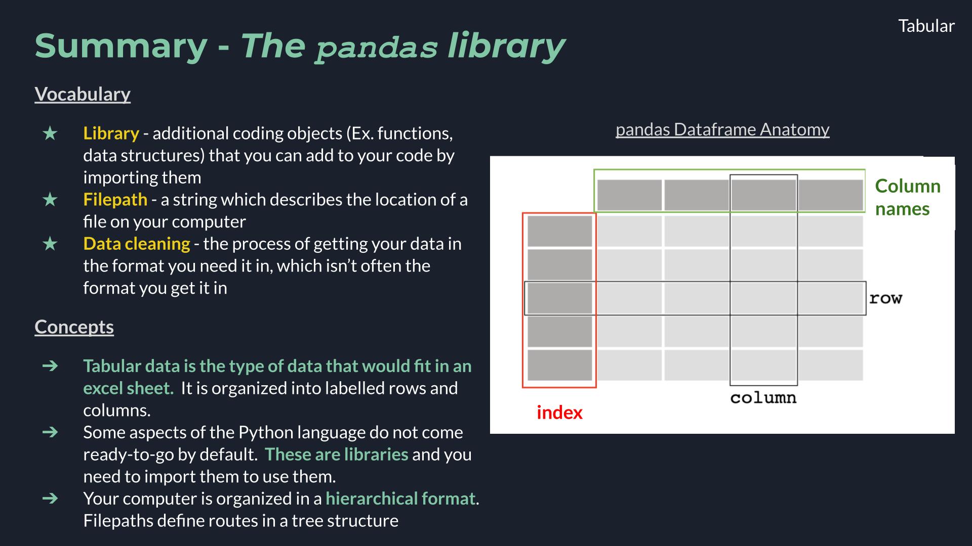
A pandas dataframe is a data structure organized into rows and columns. Other important parts of the anatomy of a data frame are the columns names and the index.

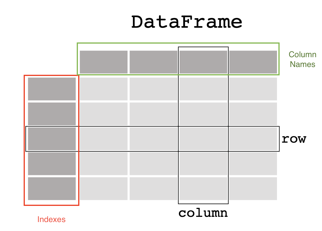
Image ammended from pandas documentation.

Here’s how we can make one from a little bit of scratch data.

# Step 1 - Define our fake data with a dictionary
forecast_dict = {
    'temperature': [25, 20, 27, 31], 
    'humidity': [60, 65, 62, 80],
    'wind_speed': [10, 9, 10, 6]
}

# Step 2 - use `pd.DataFrame()` to convert our dictionary into a dataframe
# Assign it to a variable called `forecast`
forecast = pd.DataFrame(forecast_dict)

# View the dataframe
forecast

	temperature	humidity	wind_speed
0	25	60	10
1	20	65	9
2	27	62	10
3	31	80	6

Our first dataframe! We can see that we have 3 columns, with column names temperature, humidity, and wind_speed. We have 4 data entries, or 4 rows, labeled by our indexes, which in this case are just the numbers 0-3.

📝 Check your understanding

Label the boxed components of the dataframe.

Answers reference the figure in the order: green, purple, red, orange

a) (1) 1 row of data, (2) data series, (3) column names, (4) indexes

b) (1) indexes, (2) data series, (3) 1 row of data, (4) column names

c) (1) indexes, (2) 1 row of data, (3) data series, (4) column names

d) (1) column names, (2) data series, (3) 1 row of data, (4) indexes

e) (1) column names, (2) 1 row of data, (3) data series, (4) indexes

snow_report = {
    'new_snow': [6, 4, 0, 3], 
    'snow_water_equivalent': [0.33, 0.6, 0.52, 0.7],
    'base_depth': [42, 50, 50, 37]
}
pd.DataFrame(snow_report)

	new_snow	snow_water_equivalent	base_depth
0	6	0.33	42
1	4	0.60	50
2	0	0.52	50
3	3	0.70	37

pd.Series

The other major pandas data strucutre is a Series, which represents just a single column of a dataframe. It still has indexes, like a dataframe, but since a series is only ever a single column it doesn’t have a column name.

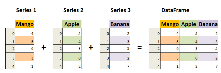
Image from Data Science Made Simple.

We access a single series (column) of our dataframe using brackets and the name of the column.

# Viewing a series (column) of data from a dataframe.
forecast['humidity']

0    60
1    65
2    62
3    80
Name: humidity, dtype: int64

Accessing values in pd.DataFrame()

Even though pandas dataframes are new data structures, some of the patterns for accessing data are very similar to what we saw in the list and dictionary data structures. What’s exciting is that the concept – indexing – is conceptually similar and so in response the syntax is also similar.

Two main ways you may want to access data in a dataframe might be:

1. look at all the data in a single column

2. look at all the data in a single row

View data in a single column

The syntax for this is akin to looking up an item in a dictionary:

forecast['humidity']

0    60
1    65
2    62
3    80
Name: humidity, dtype: int64

View data in a single row (indexing)

When looking up data for a row we use the indexes, and the same [] syntax that we have seen in lists. pandas uses the [] and : notation in the exact same way. The only new addition is the .iloc syntax that goes before the square brackets [].

# Display just the row of index 2
forecast.iloc[2]

temperature    27
humidity       62
wind_speed     10
Name: 2, dtype: int64

# Display rows index 2-3
forecast.iloc[2:4]

	temperature	humidity	wind_speed
2	27	62	10
3	31	80	6

The checkins below use the forecast dataframe we have been working with.

forecast = pd.DataFrame({
    'temperature': [25, 20, 27, 31], 
    'humidity': [60, 65, 62, 80],
    'wind_speed': [10, 9, 10, 6]
})

forecast

	temperature	humidity	wind_speed
0	25	60	10
1	20	65	9
2	27	62	10
3	31	80	6

📝 Check your understanding

1. Write a line of code to get just the wind_speed column.

2. Write a new line of code to get just the row of index 3.

📝 Check your understanding

What is the value of forecast['humidity'].iloc[2]?

a) the row: 27 62 10

b) the column: 60 65 62 80

c) the row: 20 65 9

d) 65

e) 62

🌟 A note about assigning dataframes to variables

It’s easy to feel like when you do something to find one part of a dataframe (Ex. forecast.iloc[2:4] or forecast['humidity']) you have changed the dataframe. This is not the case, however, and the original dataframe stays the same.

# Looking up the 2nd and 3rd indices of the forecast dataframe
forecast.iloc[2:4]

	temperature	humidity	wind_speed
2	27	62	10
3	31	80	6

# `forecast` is still the same dataframe
forecast

	temperature	humidity	wind_speed
0	25	60	10
1	20	65	9
2	27	62	10
3	31	80	6

This is nice for data exploration, when you don’t want the values to change every time you look at them. If you are trying to permanently change your data, you need to remember to update the dataframe by reassigning the variable.

# Updating the forecast variable with just the two rows
forecast = forecast.iloc[2:4]

# `forecast was updated`
forecast

	temperature	humidity	wind_speed
2	27	62	10
3	31	80	6

Using some real data❗️

To work with the pandas library we’ll use as an example some USGS stream gauge data (Source link).

First let’s open up the file. We aren’t going to dive into this too much so right now just notice that the function I used is pd.read_csv() (docs).

# Read in the data
water_vars = pd.read_csv('./data/englewood_3_12_21_usgs_water.tsv', sep='\t', skiprows=30)

# Check it out 👀
water_vars

	agency_cd	site_no	datetime	...	210924_00300_cd	210925_00400	210925_00400_cd
0	5s	15s	20d	...	10s	14n	10s
1	USGS	06711565	2021-03-12 00:00	...	P	8.1	P
2	USGS	06711565	2021-03-12 00:15	...	P	8.1	P
3	USGS	06711565	2021-03-12 00:30	...	P	8.1	P
4	USGS	06711565	2021-03-12 00:45	...	P	8.1	P
...	...	...	...	...	...	...	...
142	USGS	06711565	2021-03-13 11:15	...	P	7.9	P
143	USGS	06711565	2021-03-13 11:30	...	P	7.9	P
144	USGS	06711565	2021-03-13 11:45	...	P	7.9	P
145	USGS	06711565	2021-03-13 12:00	...	P	7.9	P
146	USGS	06711565	2021-03-13 12:15	...	P	7.9	P

147 rows × 12 columns

Option 2: This piece of code below also works and is more specialized to tab-seperated sheets. I chose to use the more generalized read_csv function above.

df = pd.read_table('./data/englewood_3_12_21_usgs_water.tsv', skiprows=31)

Filepaths

Your computer is organized hierarchically.

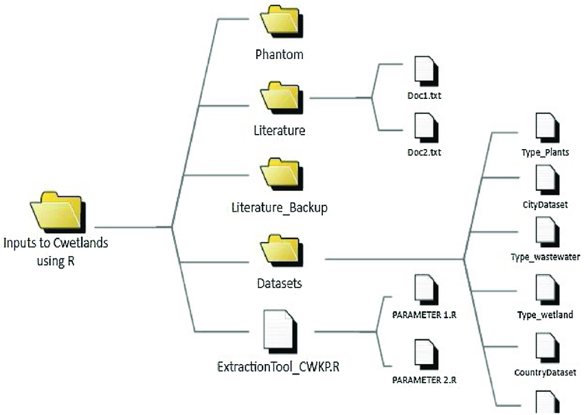
Figure from ResearchGate

The other part of that data loading statement to take note is the './data/englewood_3_12_21_usgs_water.tsv' part. This is called the filepath and it is a string that describes the location of the data that you want to open. A few pieces of the anatomy of a filepath to notice:

• / - forward slashes signal that you have entered a new folder. (Windows machines natively use a back slash \, but the Anaconda powershell can handle either)

• .tsv - this is the file extension, which tells us what type of file format the data is stored in an informs us how we open it

• . - the period at the beginning tells the computer to start looking for data in the same place that the code is being run in.

Choosing to start your filepath with a . is called specificying a relative filepath, because you are telling the computer to start looking for the file relative to where the file is being run. If you move this file to another place on your computer and don’t move the data with it the import statment won’t work anymore. The alternative to a relative filepath is an aboslute filepath, in which case you start your file path at the very tippy top of your computer’s organizational structure (the root directory).

Other vocab notes:

• directory is the same thing as a folder.

To loop back to our example, we put together our filepath by defining the following directions for our computer:

1. start by specifing the current directory as the starting point: .

2. go into the data folder: ./data

3. choose the file named englewood_3_12_21_usgs_water.tsv: './data/englewood_3_12_21_usgs_water.tsv'

🎉 And there we have our file

📝 Check your understanding

Say you are working in the folder structure shown in the image above.

What is the absolute relative filepath from the code file PARAMETER2.R to the data file CountryDataset?

Back to our data

This data isn’t super meaningful at first glance. In the block of code below I do some formatting to improve that. This step is often called data cleaning is unfortunately pretty common with real world data. You will likely spend a chunk of your time on this. (This is sometimes refered to as the 80/20 rule for data science and there is a lot of chatter that goes into trying to reverse it).

That isn’t the focus right now, though. I want to get onto working with the data so I’ve smushed all these lines of code together. I left comments so if you want to come back later to break this into seperate code blocks and see what I did you can.

# There are a lot of variables here, so let's shorten our dataframe to a few variables
water_vars = water_vars[['datetime', '210920_00060', '210922_00010', '210924_00300', '210925_00400']]
# Get rid of the first row of hard-coded datatype info
water_vars = water_vars.drop(0)
# Rename the columns from their USGS codes to more human-readible names
name_codes = {'210920_00060': 'discharge','210922_00010': 'temperature', '210924_00300': 'dissolved oxygen', '210925_00400': 'pH'}
water_vars = water_vars.rename(columns=name_codes)
# Convert columns with numbers to numeric data types
water_vars = water_vars.apply(pd.to_numeric, errors='ignore', axis=1)

Our cleaned version of the data:

water_vars

	datetime	discharge	temperature	dissolved oxygen	pH
1	2021-03-12 00:00	44.5	8.1	8.3	8.1
2	2021-03-12 00:15	44.5	8.1	8.2	8.1
3	2021-03-12 00:30	44.5	8.1	8.2	8.1
4	2021-03-12 00:45	44.5	8.1	8.1	8.1
5	2021-03-12 01:00	44.5	8.1	8.1	8.1
...	...	...	...	...	...
142	2021-03-13 11:15	42.6	6.7	9.8	7.9
143	2021-03-13 11:30	42.6	6.7	9.9	7.9
144	2021-03-13 11:45	42.6	6.7	10.2	7.9
145	2021-03-13 12:00	46.5	6.7	10.3	7.9
146	2021-03-13 12:15	NaN	6.6	10.3	7.9

146 rows × 5 columns

Accessing larger data

Our example dataframes from the previous section were small enough that we could always see the whole thing just by printing it. That won’t usually be the case with real data.

When the data is long there are other ways besides reading through it all to help you get a sense of the data. One way is to get some overview statistics with the .info() or the .describe() methods.

.info() returns:

• data type and number of indexes

• index values

• columns with number of non-null values and data type

• how much memory the object uses

water_vars.info()

<class 'pandas.core.frame.DataFrame'>
RangeIndex: 146 entries, 1 to 146
Data columns (total 5 columns):
 #   Column            Non-Null Count  Dtype 
---  ------            --------------  ----- 
 0   datetime          146 non-null    object
 1   discharge         145 non-null    object
 2   temperature       144 non-null    object
 3   dissolved oxygen  146 non-null    object
 4   pH                146 non-null    object
dtypes: object(5)
memory usage: 5.8+ KB

for each column .describe() returns:

• “count” - number of non-null values

• “unique” - number of different values

• “top” - most common value

• “freq” - how often the most common value occurs

water_vars.describe()

	datetime	discharge	temperature	dissolved oxygen	pH
count	146	145	144	146	146
unique	146	6	20	47	5
top	2021-03-12 00:00	44.5	7.7	8.2	7.9
freq	1	52	18	24	55

🌀 More Info: Viewing more rows

By default Jupyter will shorten the data and tell you that it has done that by putting the row of ... in the middle. If you would like to change the default to show more rows or columns you can do that with:

# Here 20 is the number of rows you would like to display
pd.set_option('display.max_rows', 20)

Aggregations

Another way to get a sense of your data is to run a few aggregations on the data, such as taking the max or min of specific columns. You also might need to do this as a part of your research. Some common aggregations:

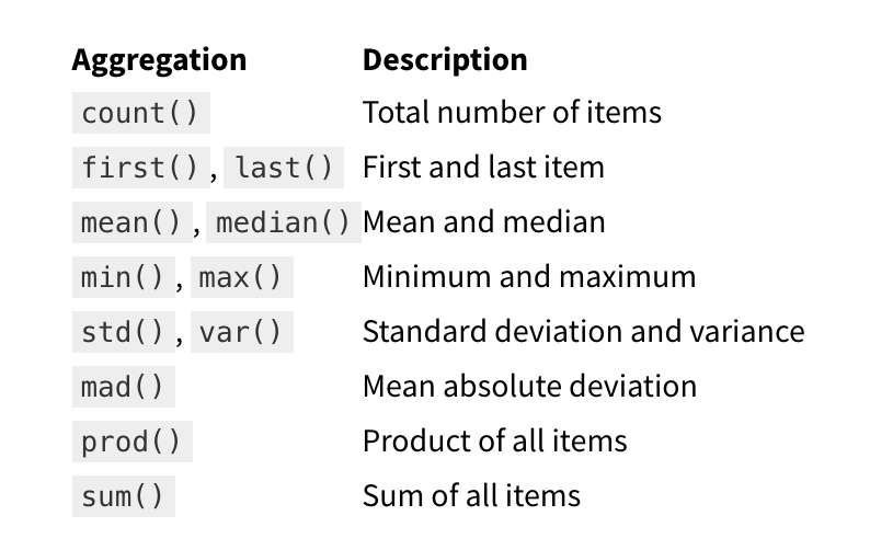
Table from jakevdp’s Python Data Science Handbook

water_vars

	datetime	discharge	temperature	dissolved oxygen	pH
1	2021-03-12 00:00	44.5	8.1	8.3	8.1
2	2021-03-12 00:15	44.5	8.1	8.2	8.1
3	2021-03-12 00:30	44.5	8.1	8.2	8.1
4	2021-03-12 00:45	44.5	8.1	8.1	8.1
5	2021-03-12 01:00	44.5	8.1	8.1	8.1
...	...	...	...	...	...
142	2021-03-13 11:15	42.6	6.7	9.8	7.9
143	2021-03-13 11:30	42.6	6.7	9.9	7.9
144	2021-03-13 11:45	42.6	6.7	10.2	7.9
145	2021-03-13 12:00	46.5	6.7	10.3	7.9
146	2021-03-13 12:15	NaN	6.6	10.3	7.9

146 rows × 5 columns

water_vars.max()

---------------------------------------------------------------------------
TypeError                                 Traceback (most recent call last)
Cell In[26], line 1
----> 1 water_vars.max()

File ~/miniconda3/envs/sarp/lib/python3.10/site-packages/pandas/core/generic.py:11646, in NDFrame._add_numeric_operations.<locals>.max(self, axis, skipna, numeric_only, **kwargs)
  11627 @doc(
  11628     _num_doc,
  11629     desc="Return the maximum of the values over the requested axis.\n\n"
   (...)
  11644     **kwargs,
  11645 ):
> 11646     return NDFrame.max(self, axis, skipna, numeric_only, **kwargs)

File ~/miniconda3/envs/sarp/lib/python3.10/site-packages/pandas/core/generic.py:11185, in NDFrame.max(self, axis, skipna, numeric_only, **kwargs)
  11178 def max(
  11179     self,
  11180     axis: Axis | None = 0,
   (...)
  11183     **kwargs,
  11184 ):
> 11185     return self._stat_function(
  11186         "max",
  11187         nanops.nanmax,
  11188         axis,
  11189         skipna,
  11190         numeric_only,
  11191         **kwargs,
  11192     )

File ~/miniconda3/envs/sarp/lib/python3.10/site-packages/pandas/core/generic.py:11158, in NDFrame._stat_function(self, name, func, axis, skipna, numeric_only, **kwargs)
  11154     nv.validate_stat_func((), kwargs, fname=name)
  11156 validate_bool_kwarg(skipna, "skipna", none_allowed=False)
> 11158 return self._reduce(
  11159     func, name=name, axis=axis, skipna=skipna, numeric_only=numeric_only
  11160 )

File ~/miniconda3/envs/sarp/lib/python3.10/site-packages/pandas/core/frame.py:10519, in DataFrame._reduce(self, op, name, axis, skipna, numeric_only, filter_type, **kwds)
  10515     df = df.T
  10517 # After possibly _get_data and transposing, we are now in the
  10518 #  simple case where we can use BlockManager.reduce
> 10519 res = df._mgr.reduce(blk_func)
  10520 out = df._constructor(res).iloc[0]
  10521 if out_dtype is not None:

File ~/miniconda3/envs/sarp/lib/python3.10/site-packages/pandas/core/internals/managers.py:1534, in BlockManager.reduce(self, func)
   1532 res_blocks: list[Block] = []
   1533 for blk in self.blocks:
-> 1534     nbs = blk.reduce(func)
   1535     res_blocks.extend(nbs)
   1537 index = Index([None])  # placeholder

File ~/miniconda3/envs/sarp/lib/python3.10/site-packages/pandas/core/internals/blocks.py:339, in Block.reduce(self, func)
    333 @final
    334 def reduce(self, func) -> list[Block]:
    335     # We will apply the function and reshape the result into a single-row
    336     #  Block with the same mgr_locs; squeezing will be done at a higher level
    337     assert self.ndim == 2
--> 339     result = func(self.values)
    341     if self.values.ndim == 1:
    342         # TODO(EA2D): special case not needed with 2D EAs
    343         res_values = np.array([[result]])

File ~/miniconda3/envs/sarp/lib/python3.10/site-packages/pandas/core/frame.py:10482, in DataFrame._reduce.<locals>.blk_func(values, axis)
  10480     return values._reduce(name, skipna=skipna, **kwds)
  10481 else:
> 10482     return op(values, axis=axis, skipna=skipna, **kwds)

File ~/miniconda3/envs/sarp/lib/python3.10/site-packages/pandas/core/nanops.py:158, in bottleneck_switch.__call__.<locals>.f(values, axis, skipna, **kwds)
    156         result = alt(values, axis=axis, skipna=skipna, **kwds)
    157 else:
--> 158     result = alt(values, axis=axis, skipna=skipna, **kwds)
    160 return result

File ~/miniconda3/envs/sarp/lib/python3.10/site-packages/pandas/core/nanops.py:421, in _datetimelike_compat.<locals>.new_func(values, axis, skipna, mask, **kwargs)
    418 if datetimelike and mask is None:
    419     mask = isna(values)
--> 421 result = func(values, axis=axis, skipna=skipna, mask=mask, **kwargs)
    423 if datetimelike:
    424     result = _wrap_results(result, orig_values.dtype, fill_value=iNaT)

File ~/miniconda3/envs/sarp/lib/python3.10/site-packages/pandas/core/nanops.py:1094, in _nanminmax.<locals>.reduction(values, axis, skipna, mask)
   1092         result = np.nan
   1093 else:
-> 1094     result = getattr(values, meth)(axis)
   1096 result = _maybe_null_out(result, axis, mask, values.shape)
   1097 return result

File ~/miniconda3/envs/sarp/lib/python3.10/site-packages/numpy/core/_methods.py:41, in _amax(a, axis, out, keepdims, initial, where)
     39 def _amax(a, axis=None, out=None, keepdims=False,
     40           initial=_NoValue, where=True):
---> 41     return umr_maximum(a, axis, None, out, keepdims, initial, where)

TypeError: '>=' not supported between instances of 'str' and 'float'

That is a long error, but what it is telling us is that we have strings in our columns that are otherwise full of numbers, or floats. To find the max values we will need to first drop the nan values with .dropna().

water_vars.dropna().max()

datetime            2021-03-13 12:00
discharge                       48.5
temperature                      8.5
dissolved oxygen                 9.9
pH                               8.2
dtype: object

📝 Check your understanding

1. how many null items are there in the temperature column?

2. what is the most common dissolved oxygen value?

3. print the standard deviation of all of the columns of the water_vars dataframe